How to fill gaps between air quality monitoring stations
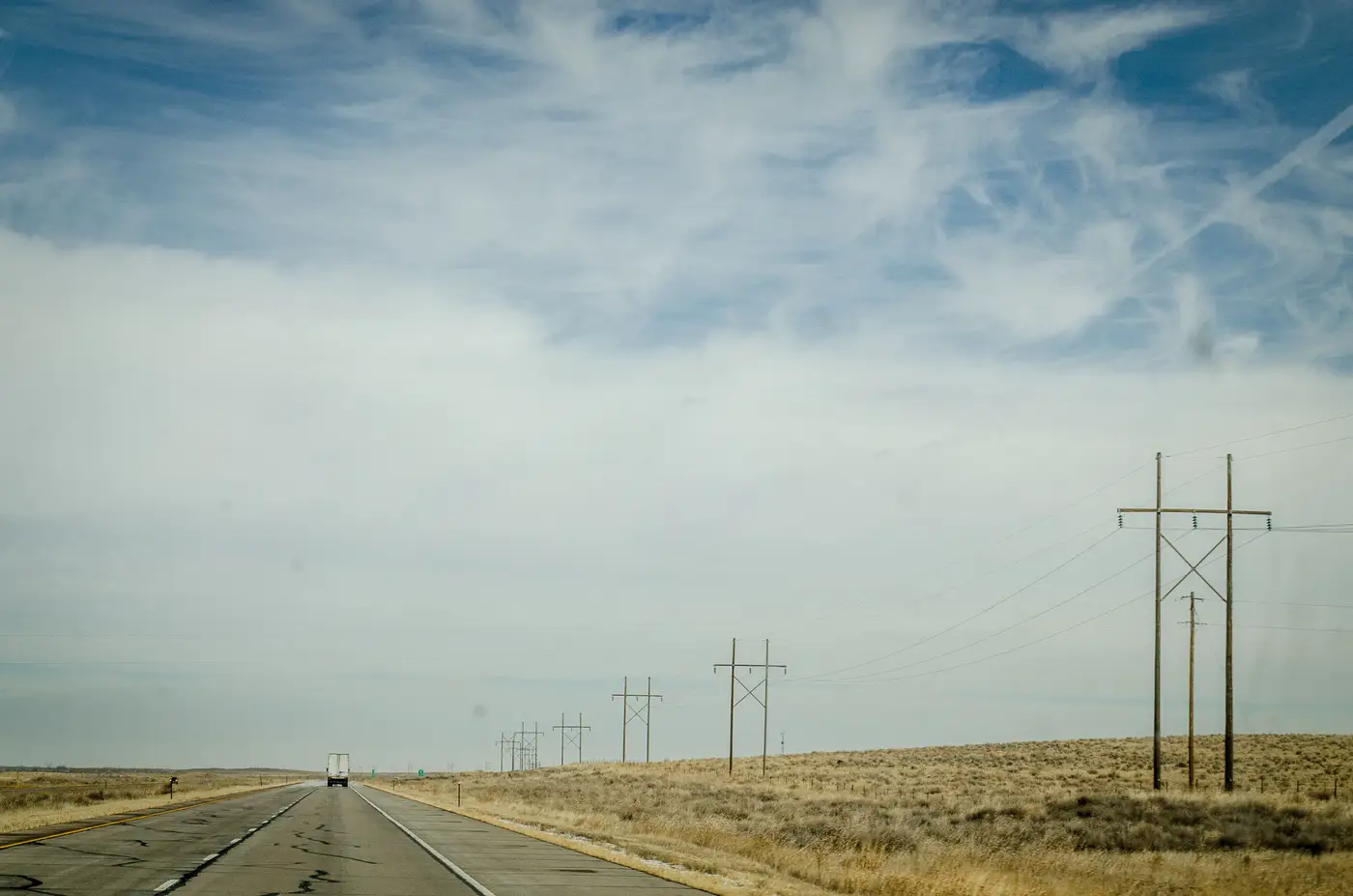
Every state network has the same problem once you look at a siting map next to a population map. The monitors cluster where the Part 58 minimums and historical exceedances put them, and the space in between gets covered by assumption. An analyst doing a five-year network assessment knows this stretch of highway, that industrial corridor, or the county without a single FRM site is a blind spot. A monitor costs money to site, certify, and run, and there's a limit to how many an agency gets to operate.
The real work is deciding what to do about the space between the stations you have.
Interpolation gets you partway
The standard move is spatial interpolation: inverse distance weighting, kriging, or a land-use regression model that pulls in traffic counts, elevation, and point-source emissions to predict concentrations at unmonitored locations. These methods work reasonably well for pollutants that behave smoothly across a region, and they're the backbone of a lot of EPA downscaler products and state-level exposure estimates used for SIP modeling.
The limits show up fast in terrain. A kriging surface built from stations thirty miles apart doesn't know about a valley that pools haze overnight or a ridge that blocks dispersion from an upwind source. It smooths right over the kind of local event that actually drives an exceedance day. Land-use regression does better at capturing those static features, but it's still working from a snapshot in time. It tells you where pollution tends to concentrate, not what's happening on a Tuesday afternoon when a wildfire plume drifts through a county with no sensor in it.
Dispersion and chemical transport models add the physics interpolation lacks. CMAQ runs, AERMOD plumes, these give you a mechanistic picture of how emissions move given the day's meteorology. They're the right tool when you need to attribute a concentration to a source. They're also heavy to run, dependent on emission inventory quality, and not something you're refreshing daily just to check whether something is building over an unmonitored stretch of the network.
Where a satellite layer fits into gap analysis
A coarse-resolution satellite pass fills a different piece of this gap. It gives you a daily look at the space the network doesn't cover. Aerosol optical depth, pulled from multispectral satellite data, doesn't give you a calibrated PM2.5 number the way an FEM instrument does. What it gives you is a relative signal, a raster showing where the column is hazier today than yesterday, gridded across your whole region instead of just at the handful of points where you've got hardware.
For network gap analysis, that's useful in a specific way. If a haze event is forming over a corridor between two stations, an AOD raster will often show the gradient building before either station's hourly data moves enough to trigger a flag. It won't tell you the exact concentration at ground level. It will tell you where to look, and sometimes that's the difference between catching an event on day one or day three. Air Quality Proxy builds that daily raster plus a per-grid-cell time series specifically for this use, so an analyst can pull the gap-area history for a siting review or a complaint investigation without waiting on a new monitor to go in.
Putting it together
None of this replaces a certified monitor, and nobody filing a SIP revision is going to cite a satellite proxy as their design value. Network gap analysis is about knowing what's happening in the space your fixed sites don't cover, so the next siting decision, complaint response, or smoke advisory is backed by something more than a guess. Interpolation gives you a modeled surface. Dispersion modeling gives you the physics. A daily AOD layer gives you eyes on the gap itself, updated every day instead of reconstructed after the fact.
If that daily between-station view is what your network assessment is missing, it's worth seeing what the raster looks like over your own region.